How to Calculate LED Voltage Drop on Long Runs

Two different things get called "LED voltage drop"

Search that phrase and half the results are about a single LED's forward voltage — the 1.8 V across a red indicator, the 3.2 V across a blue one. That is not your problem. The other half are about a run: a strip thirty or sixty meters long whose pixels are bright white near the injection point and dimmer at the far end, in slightly the wrong color.

That second thing is distribution voltage drop, and it is arithmetic. By the end of this article you will have four numbers for your own run — current per meter, the strip bus resistance, the injection spacing and the feeder gauge — plus the far-end voltage they add up to. Everything below runs on your own numbers — and says which figures to demand from your supplier. We build pixel strip at Pileds in Shenzhen, so these are the assumptions we have watched hold up on real runs.

A current-limiting resistor does not fix this: it drops voltage deliberately in series, making a far end worse.

If you are still choosing a voltage class, note that half of a sag problem is bought away at the design stage: a 24 V run wastes a quarter as much power in its copper as the same run at 12 V. That trade-off belongs to choosing the system voltage class; here the class is assumed. If "pixel" means addressable to you — WS2811, WS2812B, SK6812, one driver IC per pixel — the physics is identical to plain RGB tape, but the failure mode is nastier: a pixel that sags past its minimum supply voltage does not just dim, it lies to you.

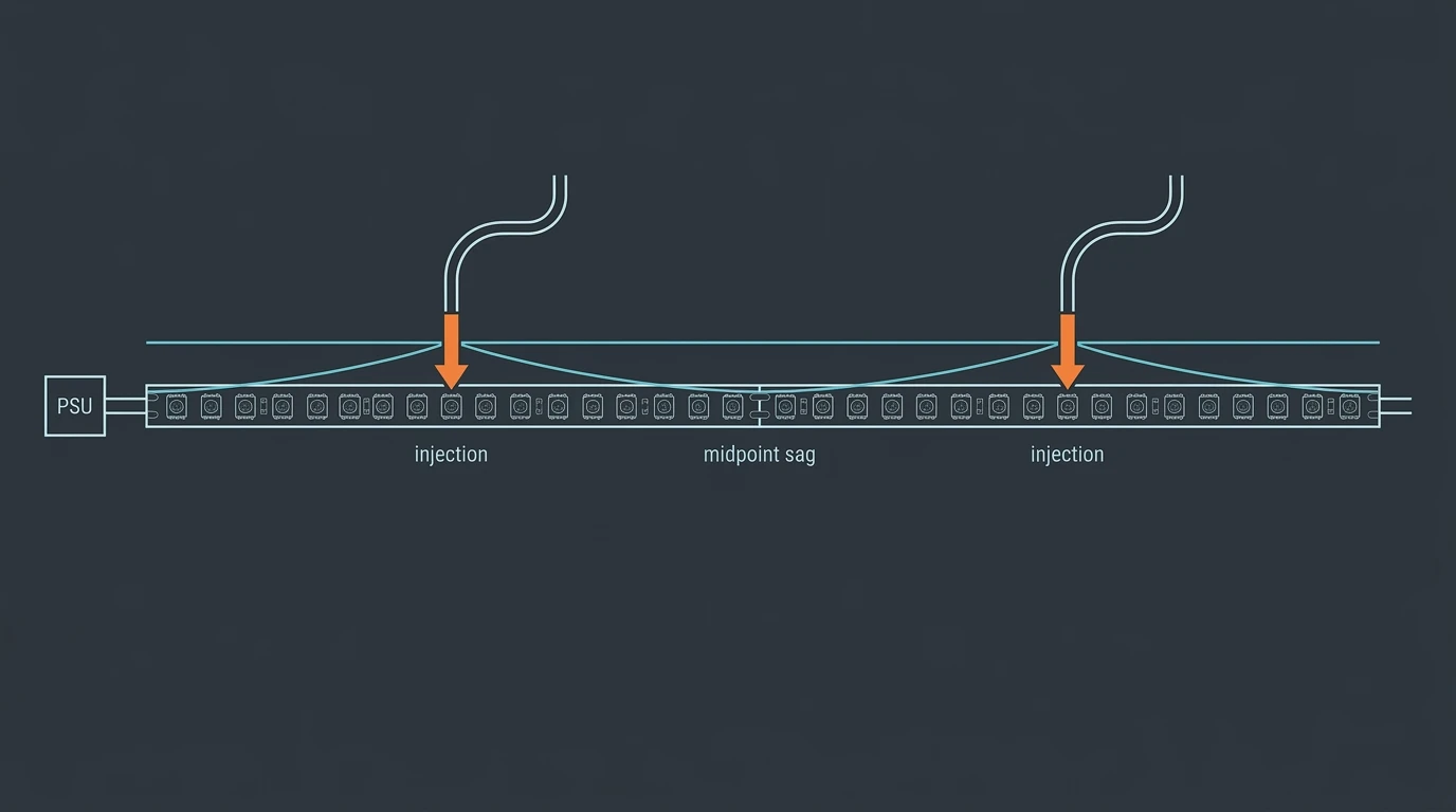
Sag is deepest at the midpoints between injection points and at the bare ends of the run — which is why "how far can I run this?" is really "how far apart do the feeds go?"

Everything below is calculated from two numbers: the current, and the resistance it crosses.

Step 1: Turn the strip's load into current per meter

Every voltage-drop calculation starts from one quantity: amps per meter — watts per meter divided by rail voltage.

Take a common 5 V addressable strip: 60 pixels per meter, WS2812B chips. Adafruit's NeoPixel powering notes put the worst case at 60 mA per pixel at full white — "up to 60 milliamps at maximum brightness white" — and they work the same example: 60 NeoPixels × 60 mA = 3.6 A. At 60 pixels per meter that is 3.6 A/m, or 18 A across a 5 m reel. Not a typo — and why 5 V pixel runs are short. The WS2811 datasheet puts its three constant-current outputs at 18.5 mA each on a 12 V rail, so the same pixel density draws 3.33 A/m: the IC family changes the load as well as the voltage.

Two rules fall out of that table:

• The worst case is white, not a color. White runs all three channels (four on RGBW) at full current at once; a saturated red frame draws roughly a third of that. Pass at full white and you pass everything.
• Doubling the rail voltage halves the current at the same wattage. White also sags more than a color, because it drives three times the current through the same copper — the LEDs' own forward voltage rising with current is second-order. Design for the full-white figure; the mixed-content figure is the floor.

Write your own number down: W/m ÷ rail voltage, or per-pixel current × pixels per meter. And settle three channels versus four first — the count changes both the current and the worst case (comparing RGB, RGBW and RGBIC pixel strips).

Step 2: Write down the resistance every meter of that current has to cross

Current leaves the supply, travels out along the positive conductor, through the strip's own copper, and returns along the negative conductor. It pays resistance twice — voltage drop exists in the supply path and the return path, as the standard treatment of voltage drop puts it. Hence the factor of two in the formulas. This is Ohm's law (V = I × R) applied to a two-conductor run: the out and return conductors sit in series with the load, so their drops add, and the resistances are the cable, the strip's copper and every joint in between. Three of them matter, and only one is the one people usually think about.

1. The feeder cable, from supply to injection point.

ΔV = 2 × R_cable × L_cable × I_total

R_cable is one conductor's resistance per meter. Copper cable resistance is published data: the American wire gauge system defines the cross-section, and standard tables list resistance per 1000 ft, which becomes Ω/m by dividing by 304.8. The table below comes from the copper wire resistance table, which gives both cold (25 °C) and warm (65 °C) values — worth having, because a cable at full load warms up and its resistance climbs with it.

Solid-conductor figures; stranded cable of the same gauge runs slightly higher. Note the shape: every three gauge steps doubles the cross-section and halves the resistance. 16 → 13 → 10 AWG is 1× → 2× → 4× the copper. When you need to halve a cable's drop, that is the lever.

2. The strip's own bus, along its length. This is the one nobody gives you. A flexible strip carries power through two thin copper lanes on the PCB, and those lanes are why the far end sags even when the feeder is oversized. You can compute it from the copper itself:

r_bus = ρ / (lane width × copper thickness)

with ρ ≈ 0.0175 Ω·mm²/m for copper at 25 °C. That is what the table above works back to: 12 AWG's 0.00531 Ω/m across 3.31 mm² implies 0.0176 Ω·mm²/m, and published copper resistivity sits in the 1.68–1.72 × 10⁻⁸ Ω·m band by temperature and temper — 1.68 for copper, 1.72 for annealed copper, both at 20 °C (resistivity reference). Run it for a good lane: 2 oz copper is 0.07 mm thick, and a 6 mm power lane gives

r_bus = 0.0175 / (6 × 0.07) = 0.042 Ω/m per conductor

Halve both the lane width and the copper weight and you quadruple the sag: against that 2 oz, 6 mm lane, a 1 oz, 3 mm lane is 0.167 Ω/m — four times worse. Halve just one of them and you double it. That ratio is why two strips with identical LEDs and wattage behave completely differently at 30 m, and why "what's your lane copper?" beats "what's the max run length?" as a supplier question. We use 0.042 Ω/m below — assume it, then replace it with your own figure, from your supplier or from a resistance measurement across a known length of strip.

3. Everything the current crosses on the way in. Connectors, terminals, solder pads and board-to-board links each add series resistance. Individually they are milliohms; across six joints and a pair of undersized pigtails they are not. There is no honest published number for this; it depends on your hardware. A 0.02 Ω joint at 6 A costs 0.12 V, which on 12 V is 1 % of your budget spent on a plug.

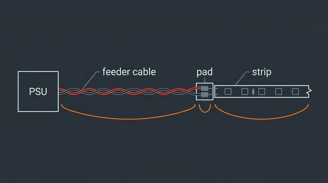
Three places volts disappear, three separate sums. Most failures come from sizing the feeder carefully and then forgetting the copper inside the strip.

A signal amplifier — the box people add when a pixel run "loses data" — fixes none of this. It re-drives the data line. If your far end is dim, the amplifier is the wrong purchase.

Step 3: Calculate the far-end voltage for your feed topology

Now put the two quantities together. Topology decides the formula — and it is where rules of thumb come from: someone ran the numbers once, and the answer hardened into folklore.

Fed from one end only. Picture the strip as a bus that sheds current along its length: at the feed it carries everything, at the far end nothing. Integrating that gives a squared law, where i is amps per meter and L the run length in meters:

ΔV_far_end = r_bus × i × L²

The ×2 for the out-and-return path and the ½ from the integration cancel exactly — hence no 2 in this formula, and r_bus must be per conductor.

Watch what the square does. A 5 V, 60 px/m, full-white strip draws 3.6 A/m; over 10 m fed from one end the formula returns 15.1 V — more than the supply itself. That is the arithmetic telling you the topology is impossible: the strip can never reach 3.6 A/m, because the far pixels would fall below their minimum supply voltage first. Shrink the run and it behaves: at 1 m the same formula gives 0.15 V (3 % of 5 V), which is why even a modest 5 V install wants its first injection close to the supply.

Fed at both ends of each segment. Inject every S meters and each point feeds S/2 meters in each direction, so the deepest sag sits at the middle of each half-segment, where the current is half the total:

ΔV_midpoint = r_bus × i × (S/2)² = r_bus × i × S² / 4

Same physics, one extra division — and it is the formula to keep in your head, because sag scales with the square of the spacing. Halve the distance between injection points and you do not halve the sag; you cut it to a quarter.

Fed from the middle. A mid-feed is two half-segments back to back: same formula, with S the distance from the feed to the next feed in each direction.

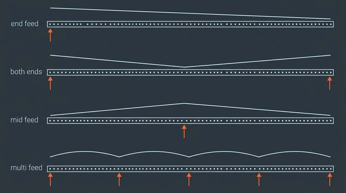
Four topologies, four sag curves. The end-fed profile is the expensive one; the multi-feed profile is what a long architectural run actually looks like.

Here is a full worked example, with every assumption in the open.

Worked example A — illustrative calculation, not a product rating. 5 V strip, 60 px/m WS2812B at full white: i = 3.6 A/m. Strip bus resistance r_bus = 0.042 Ω/m (assumed from the 2 oz / 6 mm lane above). Injection points every 1.5 m (S = 1.5 m), feeder and connectors not yet counted. >- Deepest sag in each segment: 0.042 × 3.6 × 1.5² / 4 = 0.085 V → 1.7 % of 5 V- Voltage at that point: 4.92 V, against 5.00 V at each injection point- Current through one injection point: i × S = 5.4 A

Widen the spacing and the square law bites:

Worked example B — the same calculation at 12 V and 24 V. Take a 14.4 W/m strip: i = 1.2 A/m at 12 V, 0.6 A/m at 24 V, same 0.042 Ω/m bus. Solving for a mid-segment sag of 5 % of rail voltage gives a maximum spacing of

S = 2 × √(ΔV_allow / (r_bus × i))

• 12 V: 2 × √(0.60 / (0.042 × 1.2)) = 6.9 m
• 24 V: 2 × √(1.20 / (0.042 × 0.6)) = 13.8 m

Doubling the rail voltage doubles the distance between feeds, because the current halves and the tolerable volts double. Same trade-off the voltage-class article covers from the other direction, now as arithmetic rather than opinion.

Add the feeder and the chain closes: 12 V system, supply 8 m away, a 12 A feed, 2 × R × L × I:

Those rows use the 25 °C column; a conductor at full load sits nearer the 65 °C column, which adds roughly 15 % to every figure — carry that as margin rather than ignore it.

Read that twice: moving the supply from 8 m to 3 m does more for the far end than two gauge steps usually do, and costs nothing but a longer mains lead. Distance is the cheapest lever in the calculation; copper is the expensive one. Our voltage drop and power-injection calculator applies the same feeder formula at full-load current, so you can sanity-check your own arithmetic before ordering cable.

Step 4: Pick the spacing and gauge that hold the sag inside your threshold

What number do you design to? Most published advice is either vague ("avoid noticeable voltage drop") or arbitrary ("3 %"). There are three real answers, and they are different kinds of constraint.

• The physical floor — what the driver IC still runs on. The WS2812B datasheet lists 3.5 V to 5.3 V as the absolute-maximum supply range, and characterises the part at VDD 4.5–5.5 V. So 3.5 V is the outer wall of those ratings, not a functional floor; the datasheet specifies no minimum. Treat it as a wall, never as a target.
• The visible threshold — color goes before brightness. Brightness follows current, which follows voltage, so sag dims the run; color goes earlier, because the dies do not sag equally. The same datasheet rates the red die at 2.0–2.2 V and the green and blue dies at 3.0–3.4 V, so equal sag bites blue and green first — and in practice a sagging white run drifts warm, toward brown, at the far end. Adafruit's powering notes describe the same cliff: "there's a limit below which the LED will fail to light, or will start to show the wrong color." On camera, or in a shop window, this is your binding constraint.
• The distribution guideline — 3 %, 5 %, 10 %. The 3 % figure quoted for tape lighting comes from distribution-efficiency practice, not physics: electrical codes set advisory maximum-drop guidelines — recommendations rather than enforced limits — and vary by country. On a 5 V pixel run 3 % is 0.15 V, one meter of end-fed strip. Commercial pixel practice, where the driver IC tolerates far more than a mains appliance, works to 5 % for color-critical runs and up to 10 % for decorative ones, and the pixel community's power-injection guidance is explicit that an injection wire should not exceed 10 % drop for its design current (LED strip power injection guide).

So the target is a decision: 5 % if the run will be photographed or color-matched, 10 % as the ceiling if it will not, 3 % only if the client wrote it into the spec — in which case segment more.

Now the constraint nobody mentions: the current has to enter the strip somewhere, and one injection point can only take so much — the same source puts a practical ceiling of roughly 4 A from an edge injection and 8 A from a mid injection at nominal (half-white) load, set by the strip's copper and pad geometry, not your cable.

At 5 V and full white, that ceiling, not the sag, is what stops you:

Read the 5 V row carefully: at a 5 % target the sag math allows 2.6 m between feeds, but each injection point would have to push 9.3 A, and it cannot. At 5 V the pad, not the copper, is the binding constraint — which is why 5 V pixel runs get feeds every 1–2 m in practice, and why a 30 m 5 V run looks less like a strip and more like a power distribution project. At 24 V the two constraints nearly coincide, which is why long architectural runs migrate to 24 V or to constant-current classes.

One datapoint specific to pixel runs: the ground path that carries the power current is also the data signal's reference, and the WS2812B's input threshold is a fraction of its own supply (0.7 × VDD) rather than a fixed level. A sagging strip keeps its data margin in proportion to its local supply, so a severely sagged run fails as flicker, wrong colors and dead pixels at the far end rather than as clean corruption. If you see those symptoms, measure the far-end rail before replacing the controller.

Supply tolerance is a separate question: what a 12 V rail does at 14 V is about the driver's input range, not the copper.

The same arithmetic scales to building-sized work, where the answer is a zoning plan rather than a spacing number: see spacing injection points on a curtain wall.

Step 5: Check it at the far end before you close the channel

The calculation is a prediction; ten minutes with a multimeter makes it a fact. Measure at full white, powered, running the real content — a no-load reading only tells you the supply is on.

1. Measure at the supply terminals. That is your reference; if it is already below nominal, the problem sits upstream of all of this.
2. Measure at each injection point's pads. The difference from step 1 is your feeder loss — compare it with 2 × R × L × I; if it is worse, suspect the connectors.
3. Measure at the last pixel's power pads, not the strip's end connector on the bench. That is what the sag formulas predict — and what decides whether the far end matches.
4. Note the ambient temperature: resistance rises with heat, so a cold-rig reading is optimistic — the 65 °C column above is closer to a warm install.

If the far-end figure is inside your threshold, stop — the run will look like one run. If not, the next section applies.

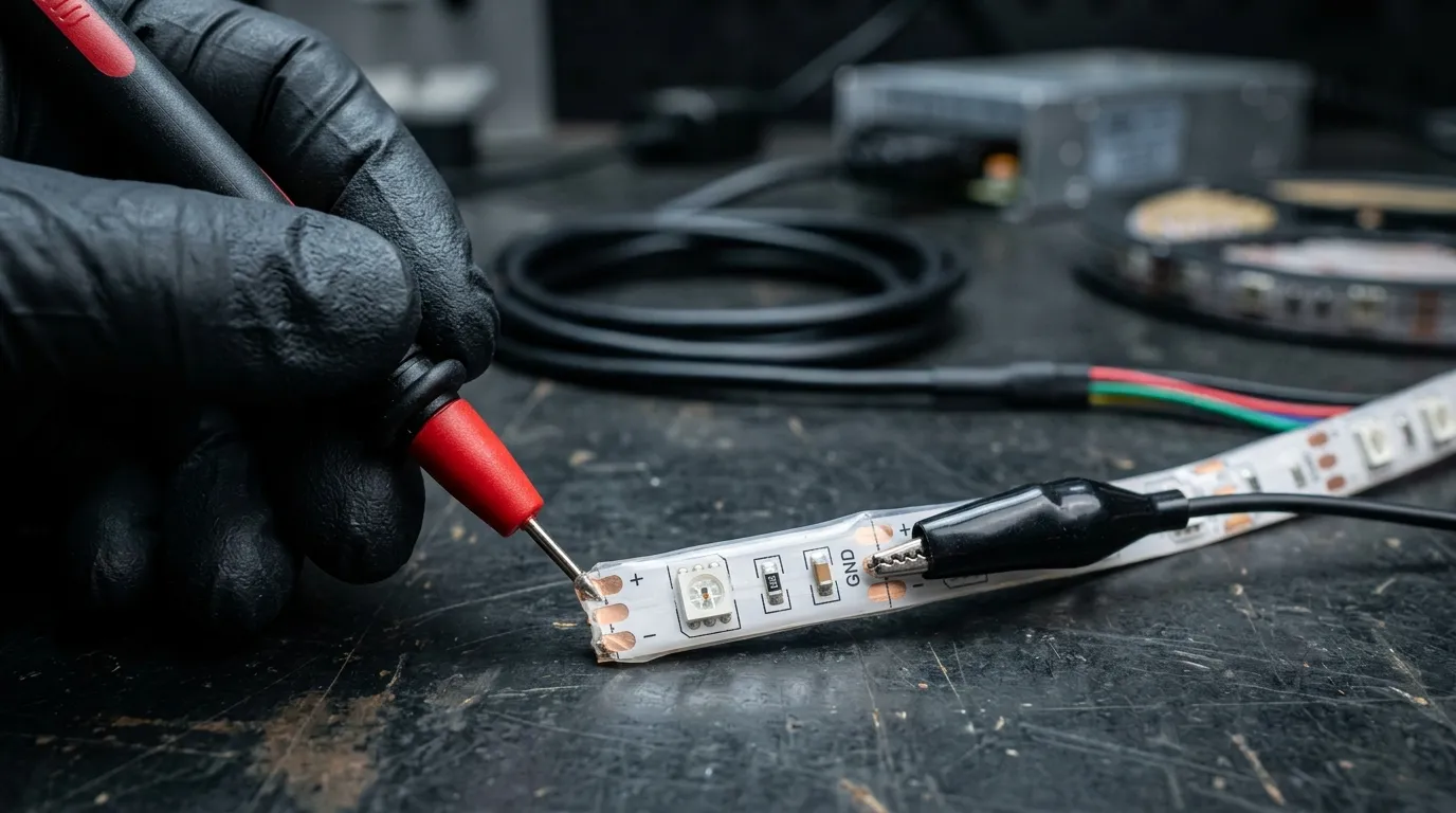
The far-end power pad at full white, under load, is the only reading that matters — every number in this article converges on it.

When the math does not fit: five ways out, in the order to try them

1. Segment the run. Add injection points until the spacing satisfies the formula. Cost: cable, connectors, a place to put the taps — and a supply sized per zone, in sizing the supply that feeds that current, which also covers the supply's own 20 % derating margin.
2. Move the supply closer. Every meter of feeder removed comes straight off the drop, with no extra copper. On a 12 V, 12 A run, 5 m of 12 AWG costs 0.64 V — 5 % of the rail spent crossing a room you may not need to cross.
3. Go up a voltage class. Same watts, less current, more tolerable volts: 24 V doubles the feasible spacing against 12 V. Free before the order; a re-order after.
4. Split into parallel runs fed from a distribution bus. Several shorter runs share the load, each fed from a bus bar or fused distribution block. Fusing on the DC side is normal practice for a reason: a shorted strip will happily ask a 40 A supply for 40 A.
5. Use a strip built for long runs. Wider lanes, heavier copper, a COB construction that lays a continuous emissive layer over that copper, a higher rail voltage or constant-current drive — all change the constants rather than the layout. A DC48V long-run class is the clearest example: same physics, a friendlier r_bus and i.

For runs long enough that low-voltage DC stops being the right answer — hundreds of meters, tunnels, mains-fed installations — the AC-versus-DC decision is worth working through before you add a third distribution cabinet. Whatever sits on the mains side of that decision is a licensed electrician's call, not a blog post's.

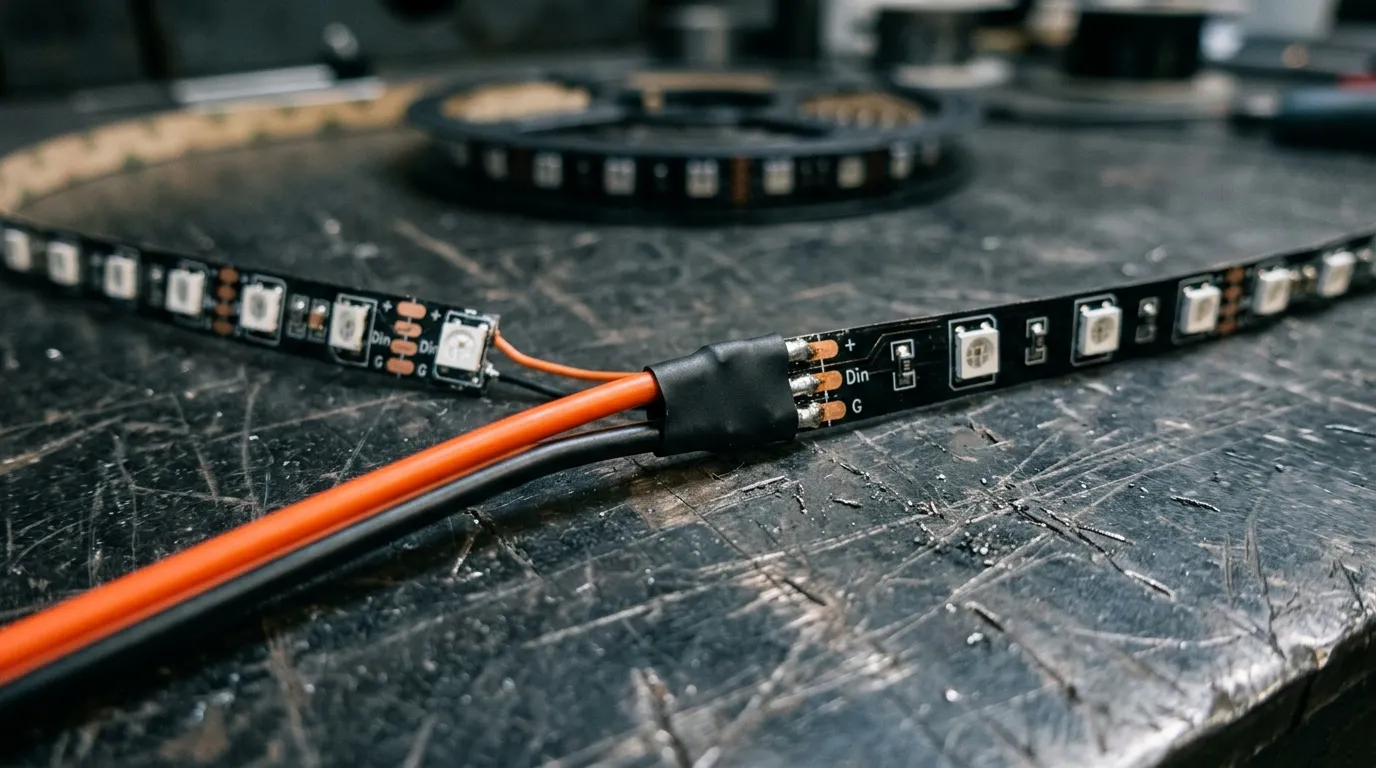
Segmenting a run in practice: a mid-run tap landing on the strip's own pads. Where that tap goes is the S in the formula — and how much current it can carry is what caps S at 5 V.

The numbers you should write on the drawing

Four figures and your run is specified:

1. Current per meter — W/m ÷ rail voltage, or per-pixel current × pixels/m. Full white, always.
2. Strip bus resistance — from the supplier, or from lane width × copper thickness. We assumed 0.042 Ω/m here; replace it with your own figure.
3. Injection spacing — S = 2 × √(ΔV_allow / (r × i)), capped by what one injection point can actually deliver.
4. Feeder gauge and length — ΔV = 2 × R × L × I, allowing for a warm conductor, supply as close as the layout allows.

The whole method: one page of arithmetic you can re-run for every layout revision rather than argue about rules of thumb. The strip at the end of it — COB and single-color lanes, DC48V long-run strip, IP68 addressable RGBW — is in the full LED strip range.

When you know your meters, your rail and your spacing, send the layout through — a second pair of eyes on a power plan is cheaper than a second purchase order.